Notes on building the simplest classification model with Perceptron

A perceptron is a simple Artificial Neural Network with a single layer that takes weighted inputs and a bias as an input and provides a binary output. The binary output can be used to classify the input features into categories.

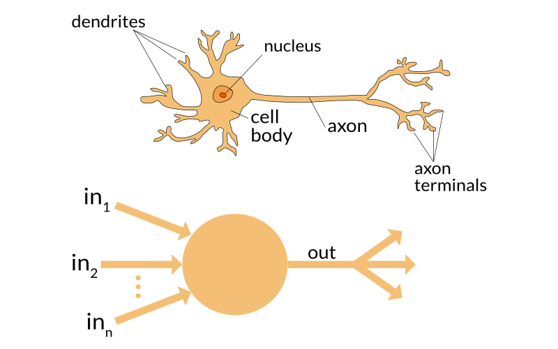
A perceptron is an algorithm modelled by how a brain cell (neuron) works.

A neuron in this context can be considered a logic gate with binary outputs. The neuron receives multiple signals at the dendrites, which then flow into the cell body and then the neuron either fires (sends signals to the output) or does not fire.

In this same way, the artificial neuron received input variables and then outputs a binary signal. The work of converting the signal to a binary output is done by a decision function.

In the perceptron algorithm, the decision function is a variation of a unit step function.

The two classes into which a perceptron classifies data should be linearly separable. If not, then perceptron may not always converge. It will keep running infinitely.

In a sense, this is similar to Linear Regression with Gradient Descenet but done in a Artificial Neural Network way.

Image from https://appliedgo.net/perceptron/ where you can go to see an implementation in Golang.

https://appliedgo.net/perceptron/

---

Intuition behind the math

The idea is to model a neuron. So we need a system that takes inputs and converts them to a binary output.

Let's look at the components of the function.

x = feature inputs

y = target outputs

decision_function = a unit step function that outputs a 0 or a 1 based on some criteria.

bias = bias is a parameter that can be thought of as the "preference" of the Perceptron. In case the bias is positive, the Perceptron would prefer classifying certain inputs to one class and vice-versa.

weights = weights are assigned to each input feature and it determines the contribution of the given input feature to the output of the Perceptron.

net_input = w1 * x1 + w2 * x2+ ... + bias

learning_rate = the rate at which adjustments are made to the weights and bias while training.

The Perceptron can be then represented as:

net_input -> decision_function -> output

---

Intuition for execution

Initialisation

We initialise the weights to random small numbers between a range from a normal distribution. (The original paper assigned initial weights as zero, but this is considered less effective than small random values)

Similarly bias can also be initialised to 0 or a small random number.

Execution

1. Take input from the input training data set.

2. Multiply input features with the weights and sum it all to have a net input.

3. Pass net input to the decision function and get an output.

4. If the output does not match the training target, adjust weights and bias as per the learning rate.

5. Perform this for all inputs.

6. Take as many iterations as defined, hopefully, it converges.

---

Implementation in Python

A simple implementation in Python:

Here is the code to train this model for the Iris dataset.

You will notice that the output chart is like this

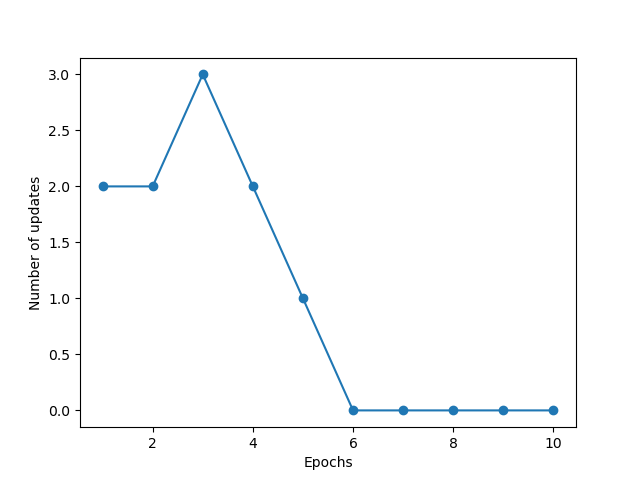
This shows how many updates are happening with each iteration. Each update represents that there were errors that the model learned and corrected.

Here you can see after the 6th iteration, the model predicted all inputs correctly.

If you change the learning rate in the training code to 0.0001, this is what happens.

Model learns slowly and never makes fully accurate predictions with Learning rate = 0.0001

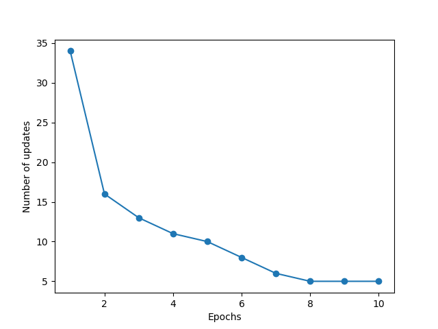
Here you can see that the model learns slowly and never reaches 0 errors in the 10 iterations we run it for.

Keep updating the learning rate (eta) and the number of iterations (n_iter) in the training code to visualise how the model learns.

That is all for today.